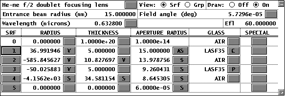
At this point, the higher-order aberrations have been significantly reduced, and the geometrical spot size, while not good enough to meet the design requirement, is much better. There is a problem in that the fifth and seventh-order aberrations are both overcorrected (positive). However, to finish the design from this point, it is better to use exact rays, which provide more flexibility in balancing all orders of aberration. The *opsetray command can be used to set up a simple ray-based error function suitable for this problem. You can change the balance between the fifth and seventh-order aberrations by changing the axial ray height between surfaces 2 and 3. Surface 2 introduces undercorrected aberration, and surface 3 introduces overcorrected aberration. The relative amount of aberration is proportional to the fifth power of the ray height for fifth-order aberration, and seventh power of the ray height for seventh-order aberration. If you increase the space between the lenses, so that the ray height drops on the overcorrecting surface, there will be less overcorrected seventh order than fifth, which is what is needed. For a starting system, choose radii of 50, 0, and -50, and add thickness 2 as a variable, so now you have a total of 4 variables.
- Modify lasrdblt.len according to the above paragraph, and execute the *opsetray command by clicking Optimize >> SCP Operands Setup >> Rays. The output should be as follows.
*opsetray (operand numbers in parentheses) Paraxial data
| PY |
PU |
PYC |
PUC |
| -- (1) |
-0.250000 (2) |
6.0000e-05 (3) |
9.6967e-07 (4) |
On-axis — YFS(10)
| FY |
DY |
OPD |
DMD |
| 0.700000 |
0.225818 (11) |
-14.364553 (12) |
-- (13) |
| 1.000000 |
0.898561 (14) |
-75.601888 (15) |
-- (16) |
| Edge of field |
6.0000e-05 YC(20) |
-9.5362e-11 YFS(21) |
-4.1666e-11 XFS(22) |
| FY |
DY |
OPD |
DMD |
| -0.700000 |
0.225817 (24) |
-14.364484 (25) |
-- (26) |
| 0.700000 |
-0.225819 (27) |
-14.364621 (28) |
-- (29) |
| FX |
DY |
DX |
|
| 1.000000 |
-8.3439e-07 (30) |
0.898561 (31) |
|
Other data 60.000000 EFL(0) -9.6934e-07 COMA(5) -3.6592e-18 DIST(6)
- To form the error function, delete the aberration operands, then use the OPD of the on-axis rays through the 0.7 and 1.0 aperture zones (OCM12 and OCM15). The OPD is proportional to the area under the ray-intercept curves, so minimizing these quantities should maximize the on-axis performance. Add a row to the spreadsheet using SHIFT+SPACE , as before, and enter the operands as shown in the following spreadsheet. Close the spreadsheet.

- After you have entered the data, save the lens under a new name (e.g. lasrdb2.len), then use the iterate toolbar icon (SHIFT+F9 ) to optimize the lens. After two cycles (20 iterations), the optimization error function should be essentially zero.
*ITERATE FULL 10
| NBR |
DAMPING |
MIN ERROR |
CON ERROR |
PERCENT CHG. |
| 0 |
0.004276 |
54.415006 |
-- |
|
| 10 |
5.4530e-08 |
0.237275 |
-- |
5.871821 |
*ITERATE FULL 10
| NBR |
DAMPING |
MIN ERROR |
CON ERROR |
PERCENT CHG. |
| 0 |
5.4530e-08 |
0.237275 |
-- |
|
| 10 |
2.3317e-12 |
1.5880e-11 |
-- |
99.819983 |
- To see the present state of correction of the system, enter the command *opsetabr in the command line. The output should be as follows.
*opsetabr (operand numbers in parentheses) Paraxial data
| PY(1) |
PU(2) |
PYC(3) |
PUC(4) |
| -- |
-0.250000 |
6.0000e-05 |
1.2608e-06 |
First-order chromatic
| PAC(6) |
PLC(7) |
SAC(8) |
SLC(9) |
| -- |
-- |
-- |
-- |
Third-order Seidel
| SA3(11) |
CMA3(12) |
AST3(13) |
PTZ3(14) |
DIS3(15) |
| -0.007374 |
9.1427e-07 |
-1.3687e-11 |
-2.0379e-12 |
1.4358e-17 |
Fifth-order Seidel
| SA5(21) |
CMA5(22) |
AST5(23) |
PTZ5(24) |
DIS5(25) |
| 0.028142 |
4.5968e-07 |
0.028142 |
8.7698e-24 |
1.1985e-29 |
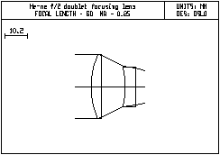
Other data 60.000000 EFL(0) -0.010215 SA7(31) 0.010553 TotalSA(41) Note that the third, fifth, and seventh-order aberrations have alternating signs, as desired. This is what a lens designer would call a solution to the design, because it works according to known principles. The spreadsheet and Autodraw window should appear as follows:


It is perhaps worth pointing out that although the above is a solution to the design task, it is not the best that could be obtained. In particular, the error function, which contains only two terms, could be expanded by adding another ray, and the image could be allowed to shift from the paraxial focus to obtain slightly better performance. For the present exercise, however, the present solution is quite adequate.
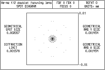
- To compare the design with the catalog lens solution obtained from in the previous section, use the on-axis spot diagram (Calculate >> Display Spot Diagram). The plot indicates that the geometrical spot size is now 0.002, a significant improvement over the previous design, and approximately equal to the diffraction limit.

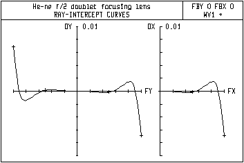
- Click Calculate >> Ray Analysis, and select Plot ray intercepts in the dialog box. The resulting ray intercept curves show that the image is at the paraxial focus, with undercorrected third-order aberration becoming important in the .2-.5 zone, overcorrected fifth-order coming in the .6-.8 zone, and undercorrected seventh-order taking over in the .9-1.0 zone.

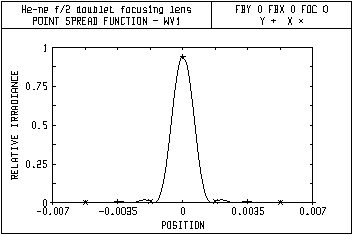
- Click Calculate >> Point Spread function, and select Plot x and y scans and Monochromatic from the dialog box. Close the box by clicking OK . The graphics window should be similar to the following.

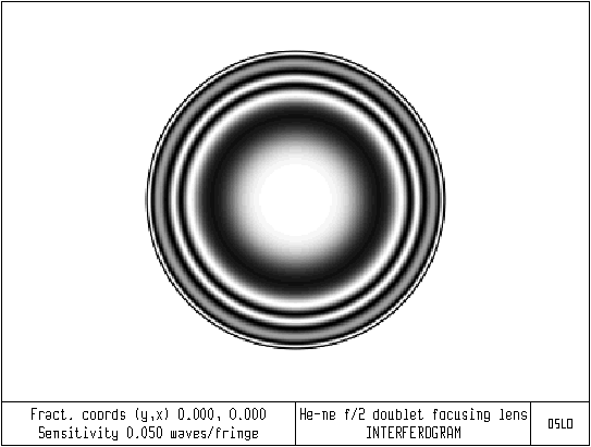
The above indicates that the design is now very good, with a Strehl definition of about 94%. In comparing it to the result from the preceding section, however, it should be remembered that this is a "paper" design using very expensive glass that would be hard to manufacture. The earlier one can simply be ordered from a catalog. The figure below shows an interferogram of the above design, made by computing a spot diagram with an aperture division factor of 200, and using the *interf star command in OSLO. The sensitivity of the interferometer was set to 0.05 waves, as indicated.
