DBLGAUSS.LEN - A DOUBLE-GAUSS OBJECTIVE

Tutorial example - Optimizing a double-Gauss objective The double-Gauss objective can serve as a starting system to illustrate the techniques for lens optimization with the GENII error function, specifically using the OSLO LT program (although the same system can be optimized similarly using any of the OSLO programs). It is assumed that the lens is to be optimized for f/2, 50mm focal length, 20 degrees field coverage, i.e. the same as the example system. The results will be different because the example system was created using a different optimization procedure. The example is presented as a series of explicit steps that you should duplicate on your computer. The OSLO user interface has been especially constructed to provide an easy-to-use interaction during optimization, if you follow the recommended procedure. As you progress through the design, you should save your lens so that you can recover to a given point rather than start over, if you make a mistake. The tutorial directory in public/len/demo contains lens files showing the design at various stages. You should expect your lens data to be similar, but not necessarily identical, to that in the tutorial files.

Starting Design (dblgauss0.len)

• Click File >> Open and open the lens public/len/demo/usrguide/dblgauss.len.
• Click File >> Save As and save the lens as private/len/dblgauss0.len. This will make a backup copy in your private directory that you can reopen if necessary.

• Click the F5 tool bar icon to open the surface data spreadsheet. Make sure that Autodraw is set to On, that the entrance beam radius is 12.5mm, the field angle 20 degrees, and the focal length 50.000041.
• Click on the aperture buttons for surfaces 1 and 11 and set the aperture specification to Not Checked.
• Click Optimize >> Variables and click on the Vary All Curvatures button. Click the OK button (or the check button in the spreadsheet) to close the Variables spreadsheet.
• Click Optimize >> GENII Error Function to enter the error function with default values (Note: If you enter the command geniierf_lt ?, OSLO will allow you to enter custom values for the default ray data). Note that the Target icon (Shift+F10) is enabled after you give the command, signifying that the lens has operands.
• Click the Target icon (Shift+F10) and observe the initial error function is 2.35.
• Close (i.e. OK) the lens (surface data) spreadsheet and immediately reopen it. This has the effect of saving the current lens to a temporary file, which you can recall using the Revert capability of OSLO (If you click Cancel in a spreadsheet, the program will prompt "Undo all changes ?"). You should always optimize a system with the lens spreadsheet open so that you can back up if something goes awry during the optimization process. Also, if the spreadsheet is open and Autodraw is on, the program will update the spreadsheet and draw a picture of the lens after each series of iterations.
• Click the Shift+F9 (Bow & Arrow) icon to iterate the design by 10 steps. Repeat this five or six times until the merit function goes down to about 1.44.
• Change the lens identification to "CV Solution".
• Click the Ray Analysis report graphics toolbar icon (Shift+F3) to display a ray trace analysis in the graphics window. Note that the lens still looks similar to the starting system, and that the ray curves, although different, are still reasonable.
• Click File >> Save As and save the lens as dblgauss1.len. If you want, you can compare your system with the lens of the same name in the public/len/demo/tutorial directory.

At this stage, we have only used curvatures as variables. This has the advantage that the system is still in the same general solution region as the starting system, and the disadvantage that the performance is not improved very much. The next stage of the design is to add the thicknesses as variables. When you add thicknesses, you must take extra care to provide boundary conditions to prevent the system from "blowing up", i.e. wandering off to a solution that is either non-physical or in a totally different solution region from the starting system.

Thickness Solution (dblgauss2.len)

• Click Optimize >> Variables. At the top of the spreadsheet, change the data fields so the air-space thickness bounds run between 0.5 and 25mm, and the glass thickness bounds run between 1 and 15mm.
• Click the Vary All Thicknesses button, then close (accept) the Variables spreadsheet.
• Close (accept) the lens spreadsheet, then immediately reopen, to provide a revert file.
• Click the Bow & Arrow (Shift+F9) icon once (only). Look at the lens picture made by Autodraw. Note that the first element is much too thin, resulting in a "feathered" edge, even though the axial thickness is within its bounds. Now look at the spreadsheet data and notice that the thickness of surface 2 is less than its minimum boundary (0.5mm). The feathered edge problem requires us to put a boundary condition on edge thicknesses, which we will do using "Edge Contact" solves. The minimum axial thickness violation requires us to put increased weight on boundary conditions.
• Click the Cancel button in the lens spreadsheet. When the program pops up the "Undo all Changes?" box, click OK in the box. The lens will be restored to its state when the spreadsheet was opened (i.e. right before the iteration). Reopen the lens spreadsheet, and note that this is so.

1. 1. Click the Thickness button for surface 1, then click Solves, and then Edge Contact. In the box that asks for the edge contact radius, enter 23.0.
   2. Click the Thickness button for surface 3, then click Solves, and then Edge Contact. In the box that asks for the edge contact radius, enter 16.0.
   3. Click the Thickness button for surface 8, then click Solves, and then Edge Contact. In the box that asks for the edge contact radius, enter 16.0.
   4. Click the Thickness button for surface 10, then click Solves, and then Edge Contact. In the box that asks for the edge contact radius, enter 22.0.
   5. Click Optimize >> Operating Conditions. Find the "Weight of boundary condition violations" field, and enter 1.0e4. This will force any boundary violations to have much more importance than other operands, and hence to be well controlled.
   6. Click OK to close the Operating conditions spreadsheet.
   7. Click OK to close the lens spreadsheet, then immediately reopen it.
   8. Click the Bow & Arrow icon about ten times, which should lower the error function to about 1.05.
   9. Change the lens identification to "CV/TH Solution".
   10. Click File >> Save As and save the lens as dblgauss2.len.
   11. Click the Ray Analysis Report Graphics (Shift + F3) icon. Note that although the error function is better than before, that the various ray curves are still not very good. In order to make the design better, it will be necessary to use different glasses.

For the design exercise in this tutorial, we will just vary the glasses in the inner doublets. After trying this, you can proceed on your own to make a final design by varying all the glasses. To vary glasses, it is necessary to first replace the catalog glasses with model glasses.

Variable Glass Solution (dblgauss3.len)

1. 1. In the lens spreadsheet, click on the glass button for surface 3, then click on Model. In the dialog boxes that appear, click OK three times to accept the Glass name, base index, and V-number for the model glass. After you have finished, note that the letter M appears on the glass button. Click the glass button for surface 3, and select Variable from the pop-up menu of actions.
   2. Repeat the above step for surfaces 4, 7, and 8.

1. 1. Click Optimize >> Variables. Select Row 21, then click the "Insert After" toolbar icon in the Variables spreadsheet. Then select Row 22, and hold down the Shift key while clicking on the row button three more times. This will create 4 new rows at the bottom of the variables spreadsheet.
   2. In the Surf column of the new rows, insert surfaces 3, 4, 7 and 8 respectively.
   3. In the Type column, insert DN for all 4 rows.

1. 1. Enter the above boundary conditions in the appropriate cells in the eight rows that specify the glass variables.
   2. Close the Variables spreadsheet, then close the lens spreadsheet and immediately reopen it.
   3. Click the Bow & Arrow toolbar icon several times until the error function decreases to about 0.47.

1. 1. Click Show >> Surface Data, then select Refractive indices and close (accept) the dialog box. The current refractive index data will appear in the Text output window. Note that the glass on surface 8 has a refractive index of 2.00 and a V-number of 50. This will be a difficult glass to match.
   2. Change the lens ID to "CV/TH/RN Solution", then click File >> Save As to save the current lens as dblgauss3.len. Close the lens spreadsheet and reopen it immediately.

The next task is to find real glasses to replace the model glasses. OSLO has a special command, accessible from the lens spreadsheet, that substitutes the nearest real glass for a model glass.

Real Glass Solution (dblgauss4.len)

• Click the glass button on surface 8, and select Fix >> Schott from the list of options. The program should offer to substitute LASFN31. Accept this suggestion. Close and reopen the lens spreadsheet. Click the Bow & Arrow icon many (~40?) times until the error function decreases to about 0.49.
• Click the glass button on surface 7, and select Fix >> Schott from the list of options. The program should offer to substitute SF9. Accept this suggestion. Close and reopen the lens spreadsheet. Click the Bow & Arrow icon until the error function decreases to about 0.50.
• Click the glass button on surface 4, and select Fix >> Schott from the list of options. The program should offer to substitute SF59. Accept this suggestion. Close and reopen the lens spreadsheet. Click the Bow & Arrow icon until the error function decreases to about 0.50.
• Click the glass button on surface 3, and select Fix >> Schott from the list of options. The program should offer to substitute LASF18A. Accept this suggestion. Close and reopen the lens spreadsheet. Click the Bow & Arrow icon until the error function decreases to about 0.70.

1. 1. Click File >> Save As to save the current lens as dblgauss4.len. Close the lens spreadsheet and reopen it immediately.
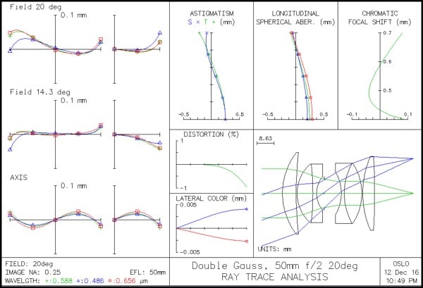
   2. Double-click the report graphics window to bring the ray analysis up to date. The curves should be similar to the following. Note that the sagittal ray-intercept curve at full field is not well controlled. Note also that the astigmatism curves at the edge of the field do not come together.

1. Open a second graphics window using Window >> Graphics >> New. Click the report graphics Through-focus MTF (Shift F6) icon. The curves should be similar to the following. Note that despite the fact that the ray analysis astigmatism curves do not come together at the edge of the field, the actual MTF curves are reasonably coincident, at least at 25 cycles/mm.

At this point, the optimization has proceeded to the point of a default solution. Now, various trials can be conducted to improve the design, such as trying additional glasses. Other possibilities for additional optimization are to remove the edge contact solves to see whether the positive elements still want to get too thin, to change the weights on selected terms in the error function, or to re-enter the error function with different rays. The general approach to optimization using OSLO is illustrated by the steps of this example: you should approach the optimization cautiously and change only a few things at a time, working interactively, until you are confident that the combination of variables and operands can be trusted to produce a system of high quality. You should always maintain a way to restore your system to an earlier state, such as using the revert capability of OSLO spreadsheets.

Final Solution (dblgauss5.len) The lens shown below (public/len/demo/tutorial/dblgauss5.len) is the result of about an hour's investigation of various options for improving the design using the GENII error function (with different weights on selected operands). It is not feasible to trace the course of this optimization explicitly. You should try to see if you can match, or improve on, the final design shown below. Note that checked apertures have been inserted to provide vignetting at the edge of the field.